Project 2: Playing with Schelling’s Segregation Model

Introduction
In this project, you will delve into the nuances and boundaries of the Schelling segregation model, a foundational model in agent-based modeling that explores how individual preferences can lead to large-scale patterns of segregation. The classic model demonstrates how even slight preferences for similar neighbors can produce significant segregation, highlighting both the power and the limitations of abstraction in social simulations.
In class, you were encouraged to critically assess this model’s assumptions and to consider more complex, real-world variables that the model omits. Aspects like the social and economic costs of mobility, the multidimensional nature of social identity, and how environmental constraints shape urban segregation patterns are just a few elements that invite further exploration beyond Schelling’s initial framework. This assignment will task you with building on the Schelling model, integrating new variables, and examining the impacts of various extensions on segregation dynamics.
Our initial starting point is the model created in class, accessible by clicking in this link.
Download the code in your computer, and make sure it runs without errors.
Step 1 - Exact Population Initialization in the Schelling Model.
In the code provided for the Schelling model, the parameter \(density\) controls the probability that any given patch will initially contain an agent. Consider \(p=density\) and \(N\) the total number of patches (the maximum population size possible).
- Adjust the model’s setup procedure so that the population includes exactly \(pN\) agents. Round the number of agents to the nearest integer as needed.
- Use the
n-ofNetLogo primitive to select specific patches on which agents (households) will be created. - Introduce a Boolean variable named
exact?to toggle between probabilistic and deterministic population sizes.
Ensure that your code is efficient and comment each step of your logic. The switch for exact? should allow you to easily switch between the two initialization modes, so test your setup by running the model in both modes to verify functionality.
Step 2 - Developing a New Segregation Metric in the Schelling Model.
In this step, you will explore a secondary metric of segregation that Schelling proposed: the proportion of agents with strictly zero neighbors of the opposite color. This metric provides insight into the degree of complete separation among groups.
- Code a New Reporter:
- Create a new global variable called
prop-uniformthat stores the proportion of agents who have zero neighbors of the opposite color. - To do this, add a new variable called
uniform?to the household agents in the code starting withhouseholds-own. This variable will be set to true if all of a household’s neighbors share its color. - For cases of low density, establish a rule to handle agents without any neighbors. Document it well.
- Create a new global variable called
- Dynamic Display:
- Add a new plot to your NetLogo model to dynamically display the
prop-uniformvalue as the model runs. - Include a monitor to collect and display the precise value of
prop-uniformat each time step.
- Add a new plot to your NetLogo model to dynamically display the
- Batch Runs:
- Conduct batch runs with 10 simulations per parameter setting, varying
similarity-thresholdfrom 0.05 to 0.75 in increments of 0.05, withdensityfixed at both 0.45 and 0.90. Use BehaviorSpace for this. Setexact?to true. - Stop each run when it reaches equilibrium or after 100 ticks. Note that this is different from what was done in class. Learn how to interpret the outputs of the BehaviorSpace in order to find how many ticks were ran before equilibrium was reached.
- Plot both
prop-uniformand the average similarity (average-similarity) of neighbors as functions of the similarity threshold for each density level. Compare these two metrics to understand if segregation patterns differ based on the metric used. Write your observations in theInfotab. As shown in class, you may use AI tools to generate the graphics.
- Conduct batch runs with 10 simulations per parameter setting, varying
I have used a prompt for ChatGPT to process my data from the table output generate by Behavior Space as follows:
This a netlogo file showing the results of a batch run of 10 simulations for each set of parameters. You must ignore the first 6 rows, as they are just metadata. The parameters I am varying for each simulation are density, exact? and similarity-threshold. [step] tells me how many time steps were ran before the simulation stabilized.Other tools I also recommend are:
When you click the Run button of BehaviorSpace it gives you 4 options of csv files to be generated. The stats csv file returns the mean and standard deviation of all runs with the same parameters combined. So maybe that’s a better option to use if all simulations run for the same amount of time.
This exercise will help you investigate different dimensions of segregation and how varying parameters influence model outcomes.
Step 3 - Quantifying Time to Equilibrium in the Schelling Model.
In this step, you will examine how the density and similarity threshold in the Schelling model influence the time it takes for the system to reach equilibrium. This will help reveal under what conditions the model converges quickly and when it struggles to stabilize.
- Explanation of High Threshold Effects:
- Begin by considering why high-density and high-threshold settings might delay equilibrium. Specifically, explain why a significant jump in the time to equilibrium is expected when the similarity threshold (
S) exceeds 50% in high-density scenarios. Write your response at theInfotab.
- Begin by considering why high-density and high-threshold settings might delay equilibrium. Specifically, explain why a significant jump in the time to equilibrium is expected when the similarity threshold (
- Batch Runs:
- Conduct batch runs of 5 simulations for each parameter combination with values of
similarity-thresholdvarying between 0.4 and 0.85 in increments of 0.05. - Fix the
densityparameter at both 45% and 90%. - Fix
exact?to true.
- Conduct batch runs of 5 simulations for each parameter combination with values of
- Recording Simulation Length:
- Track the number of ticks that have elapsed when each simulation ends. Ensure that each simulation runs until equilibrium or a maximum of 1000 time steps.
- Analysis:
- Plot the average time to equilibrium as a function of the similarity threshold for both density levels.
- Discuss how density and similarity thresholds interact to influence the time to reach equilibrium, noting any significant differences between the two density settings.
This exercise will provide insight into the Schelling model’s dynamics under different conditions, especially how specific parameter settings affect the stability of segregation patterns.
For this step, we are interested in the Step column from our table generated by Behavior Space!
Step 4 - Expanding the Neighborhood Size in the Schelling Model
In this step, you will explore how the size of an agent’s neighborhood affects the segregation dynamics in the Schelling model. Rather than focusing only on adjacent patches, agents will consider a larger area around them to evaluate their neighborhood, providing insights into the effects of neighborhood size on segregation patterns.
- Modify the Neighborhood Definition:
- Add a new parameter called
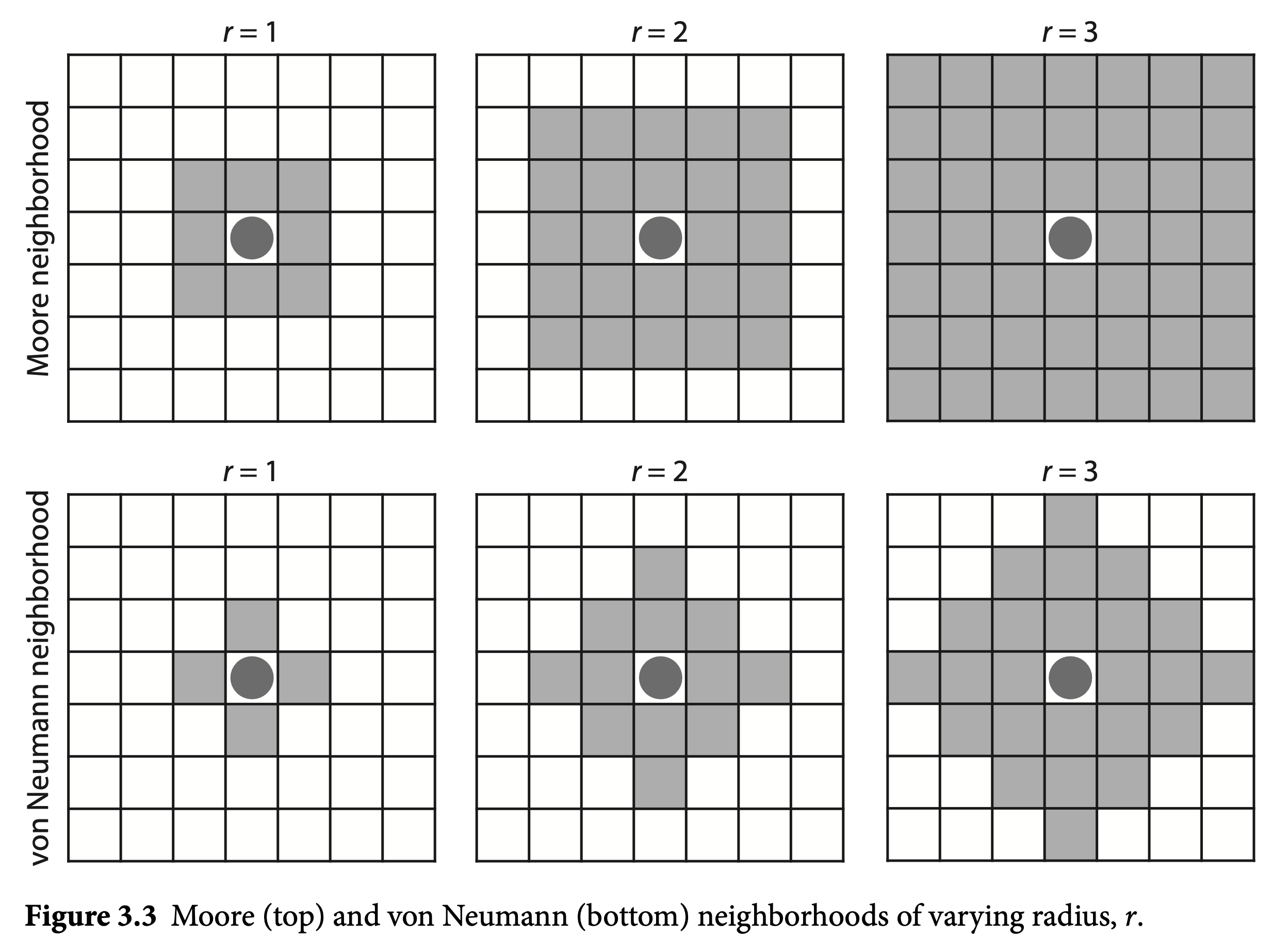
neighborhood-size, which will be an integer \(x\). You can add it as a slider or as a global variable. - This parameter will define an agent’s neighborhood as a square of width \(2x + 1\) centered on the agent (see Figure below for a visual guide). That is, for the Moore neighborhood with \(x\) (or \(r\)) equals 1, we have a square \(3x3\), while for \(x=2\) we have a square \(5x5\) with the centered agend in the middle. There is one model in the Netlogo Models Library that might be of your interest.
- Add a new parameter called
- Adjust the Model Code:
- Modify the model’s code to incorporate the
neighborhood-sizeparameter. Agents should now assess the similarity of agents within this extended neighborhood when determining whether they are “happy” with their surroundings.
- Modify the model’s code to incorporate the
- Batch Runs:
- Conduct batch runs of 10 simulations with different values of
neighborhood-size(e.g., 1, 2, 3). - Run each batch at a fixed density (e.g. \(0.5\)) and similarity threshold (e.g. \(0.5\)) to observe how changing the neighborhood size affects the model’s segregation outcomes. Set
exact?to true. - Ensure that each simulation runs until equilibrium or a maximum of 100 time steps.
- Conduct batch runs of 10 simulations with different values of
- Analysis:
- Plot the resulting levels of segregation for each neighborhood size.
- Discuss how expanding the neighborhood size influences segregation, noting any differences in segregation patterns as neighborhood size increases.
This exercise will help you explore the impact of neighborhood scope on segregation dynamics and understand how local versus extended neighborhood interactions affect social outcomes in the model.
Submission
Submit your Netlogo code on Moodle until Tuesday, November 19. Document well your code and report the answers for all the steps in the Info tab.
Grading Rubric
This project will be graded the following way: 100 pts total
- Step 1: 20 pts
- Code is correct: 10 pts
- Code is well documented: 10 pts
- Step 2: 20 pts
- Code is correct: 10 pts
- Code is well documented: 10 pts
- Step 3: 20 pts
- Code is correct: 10 pts
- Code is well documented: 10 pts
- Step 4: 20 pts
- Code is correct: 10 pts
- Code is well documented: 10 pts
- All the answers for the questions are clear and provide insightful analysis of the model: 20 pts