W₁: Components of a Model

CS300b – Agent Modeling

Eric Araújo

Communicating Your Model Clearly

What are we assuming, and what are we excluding from those assumptions?

Model Description

• Parts and properties of the model (agents, environment).
• Instantiation and initialization of the model.
• model dynamics.
• Outcome measures and data analysis techniques.

1 - Parts and Properties

• What is being represented, and what is the nature of that representation?
• If we are talking about an agent-based model, what are the agents like?
• What properties do they have?
• What behaviors do they exhibit?
• If the agents interact, how are those interactions structured?
• What is the nature of their environment, and what are its properties?

TTYN - what are the parts and properties of the particles model?

1 - Parts and Properties (example)

This model features a population of spatially embodied agents moving through continuous space, each using a coordinated walk. When agents collide, they become confused, and each sets off in a new direction. We run each model simulation for 10,000 time steps and compare the number of collisions during that time.

2 - Initialization

• What’s going on when a model simulation begins?
• How many agents are there, and what are their properties?
• Where are they in their environment and in relation to each other?
• What does the environment look like?

Research on nonlinear dynamics has shown that in complex, interconnected systems, long-term dynamics can be highly sensitive to initial conditions.

2 - Initialization (example)

A population of N agents is initialized with each agent placed at a random real-valued locations on an \(L×L\) grid with periodic boundaries. Each agent \(i\) has a direction heading \(\theta_i\), which is initially chosen at random from a uniform distribution of integers \([0, 359]\). Each agent is fully defined by its location and directional heading. Other model parameters are the whimsy, \(w\), which determines the turning angle agents use on each time step, and the speed, \(s\), which determines the size of the step they take when moving. Finally,we keep track of the cumulative number of collisions over time, \(C(t)\).

3 - Dynamics

• How does the state of the model system update from one moment to the next?
  • discrete or continuous?
  • discrete = ticks = time steps

3 - Dynamics

• What happens in one time step of a model simulation?
  • Agents take actions at the same time (synchronously) or one at a time (asynchronously)?
  • Should each agent complete all actions before the next agent is scheduled?
• This ordering of the computations performed during each time step is called scheduling.
• Specification of a model’s dynamics includes any stopping conditions for the model.
  • Fixed number of steps
  • Equilibrium

3 - Dynamics (example)

At each time step, each agent, in a random order, turns, moves, and collides. An agent first turns by adding to its direction heading an integer value that is randomly drawn from a uniform distribution in \([0, w]\). The agent then subtracts a newly drawn value from the same distribution from its directional heading. In other words, its new directional heading is \(\theta_i + \epsilon\), where \(\epsilon\) is randomly drawn from a binomial distribution bounded in \([−w,w]\). The agent then moves \(s\) units forward. If there are any other agents with a position within one unit of the focal agent’s new location (defined by the Euclidean distance between the centers of each agent), a collision occurs between the focal agent and all of these other nearby agents. In this case, all of the agents involved in the collision update their heading to a new value randomly selected from the uniform distribution \([0,359]\). Each of the involved agents then moves forward \(0.1\) spatial units in order to move away from the site of the collision and avoid cycles of perpetual collision. If a collision occurs,the cumulative collision counter \(C(t)\) is incremented by one.

4 - Outcomes

• How the model’s outcomes will be quantified and how the model’s behavior under different conditions will be characterized for comparison.

What are the outcomes for the particles model?

Reproducibility

• Share well-documented code and instructions.
• Ensure others can understand and replicate your work.

Notes: Emphasize the importance of a clear and complete model description for scientific communication.

Refer to sources and for guidance on writing model descriptions, mentioning the ODD protocol as a potential framework.

Exploration and Extensions

Beyond Particle World

• Exploration:
  • Experiment with different movement rules (will be done in HW-01).
  • Add new variables (e.g., particle size, attraction/repulsion).
• Extensions:
  • Introduce more complex environments.
  • Explore the emergence of collective behavior.
• Particle World is a stepping stone to more sophisticated ABMs!

Encourage exploration and experimentation with the Particle World model.

Suggest potential extensions to make the model more complex and realistic.

End on a note of excitement about the possibilities of ABMs.

Schelling’s Segregation Model

Schelling’s Segregation Model

Introduction

• The Puzzle of Segregation: How do segregated neighborhoods form even without overt discriminatory policies?
• Schelling’s Insight: Thomas Schelling’s model helps us understand how segregation emerges from seemingly innocuous individual preferences.
• Agent-Based Modeling: We’ll use ABM to simulate individual behavior and observe the resulting patterns.

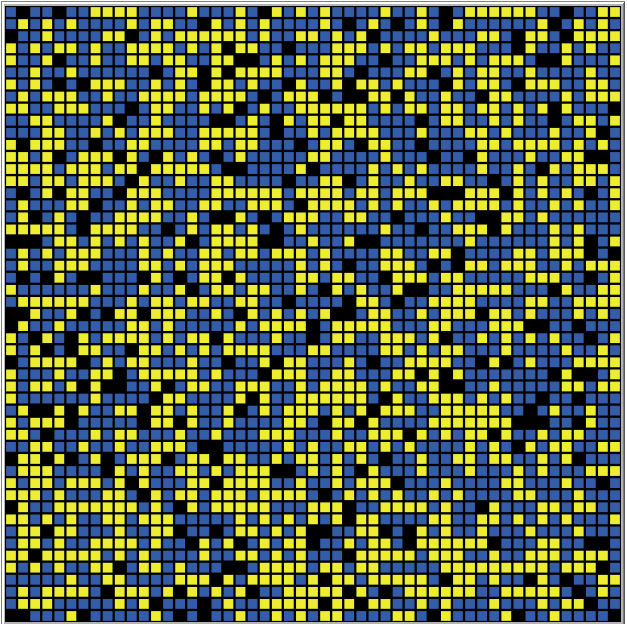
The Basic Model Setup

• Agents and Environment:
  • Agents: Individuals or households residing on a grid
  • Environment: The grid represents a city or neighborhood
• Key Parameters:
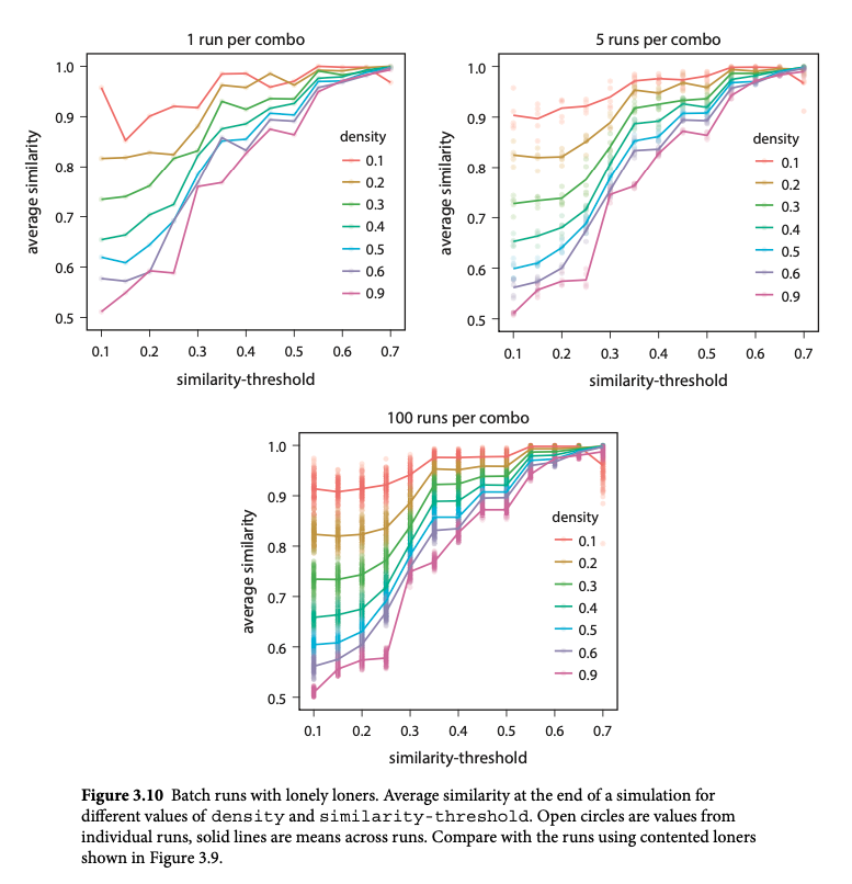
  • Population density (p): Proportion of grid cells occupied by agents
  • Similarity threshold (S): Minimum proportion of similar neighbors required for an agent to be “happy”

Visualization of the model’s initial state, with agents of two different colors randomly distributed on a grid

Agent Behavior: The Rules of the Game

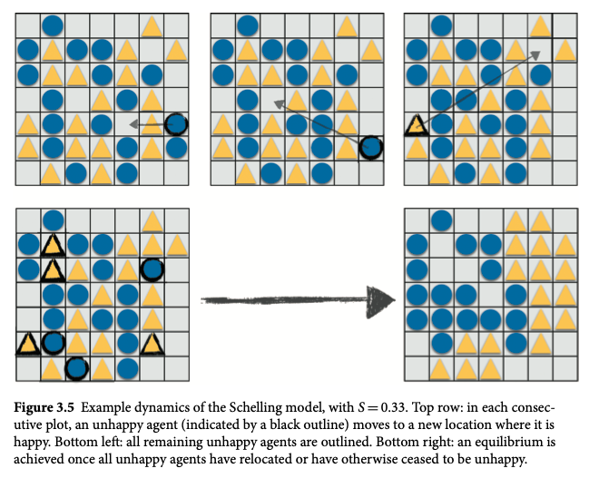
• The Happiness Rule: Agents assess their satisfaction based on the similarity threshold.
• Unhappy Agents Move: Unhappy agents relocate to empty cells where they can meet their similarity threshold.

Figure 3.5 from the book Modeling Social Behavior

Emergence of Segregation: Micromotives, Macrobehavior

• The Surprising Outcome: Even with a relatively low similarity threshold, the model consistently leads to significant segregation.
• The Power of Simple Rules: Simple individual preferences can result in complex and unexpected patterns at the societal level.

Emergence of Segregation: Micromotives, Macrobehavior

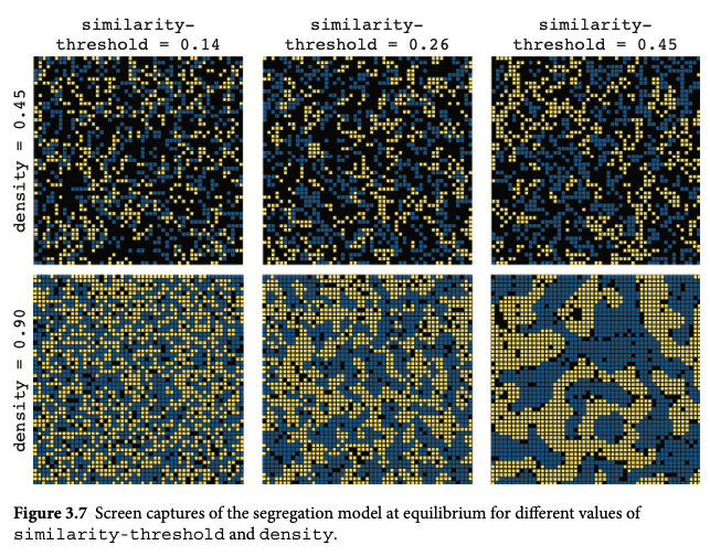
Snapshots of the model at equilibrium for different similarity thresholds and densities

Model Analysis: Beyond Visual Inspection

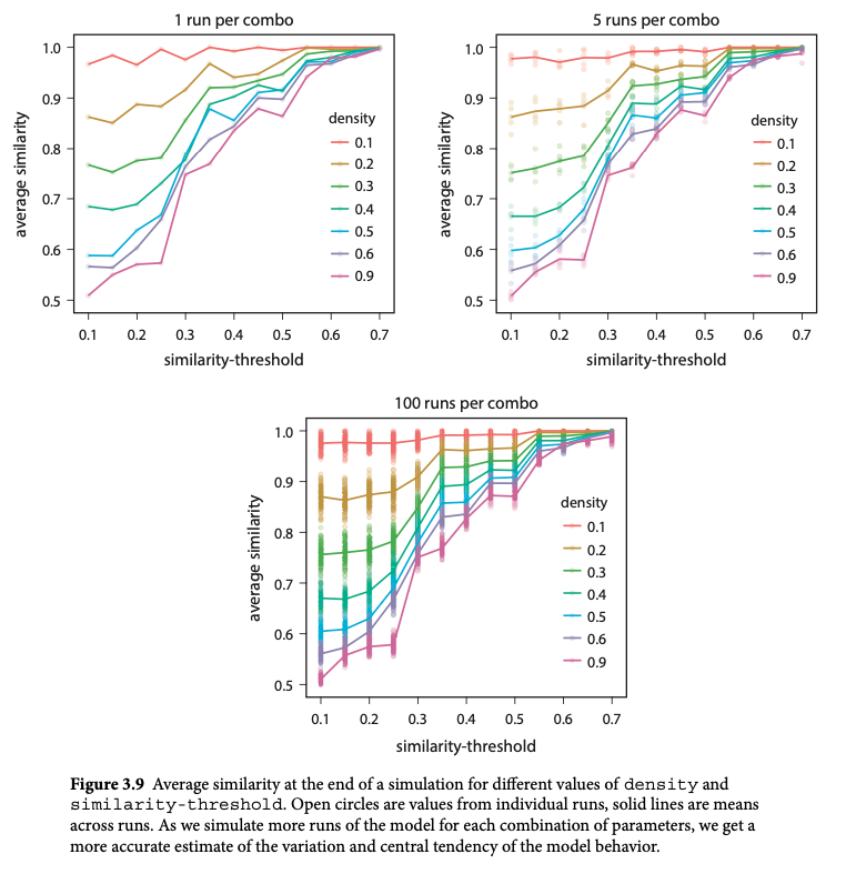
• Quantitative Measures: Analyze the model beyond visual observation using:
  • Average Similarity: Proportion of an agent’s neighbors belonging to the same group
  • Segregation Index: Metric capturing the overall level of segregation (explain the specific index used or provide a reference)
• Batch Runs and Parameter Sweeps: Use batch runs to explore the model’s behavior across a range of parameter values.

Batch Run Results and Interpretation

• Key Insights:
  • Discuss the patterns observed in the results.
  • Focus on how varying the similarity threshold and density affects the level of segregation.
• Model Limitations:
  • Acknowledge the simplifying assumptions.
  • Note the need for caution when generalizing to real-world scenarios.

Extensions and Modifications

• Contented Loners: What happens if some agents are always happy regardless of their neighbors?
• Minority-Seeking Agents: What if some agents prefer to be in the minority?
• Multiple Groups: What are the implications of having more than two groups?
• Invitation to Explore: Consider other modifications and extensions, highlighting the model’s flexibility.

Conclusion

• Key Takeaways:
  • Simple individual preferences can lead to complex patterns of segregation.
  • The level of segregation is influenced by the similarity threshold and population density.
  • Models help us understand social phenomena and explore potential interventions.

You’ll need to replace the placeholders for images and references with the actual content.

Consider adding interactive elements or animations if your presentation software supports them. For example, you could animate the movement of unhappy agents or have sliders to adjust parameters in real-time. Remember that this is a starting point, and you can adjust the content and structure to suit your needs and audience.